SPATIAL PATTERN ANALYSIS

Problem

The problem can be into six primary parts, which will be referred to as 8-1, 8-2, 8-3, 8-4, 9-1, and 9-2, respectively. 8-1, 8-2, and 8-3 involve analyzing the distribution of service calls to fire stations for a certain area. In 8-1, the problem was to analyze the spatial distribution of false alarms for a fire station, to determine if there was clustering. In 8-2, the problem was to analyze all calls for service in January 2015. In 8-3, the issue was to analyze the clustering relationships based on the distance between each point. In 8-4, the problem was to analyze library patron distribution using polygon data. In 9-1, the issue was to analyze the fire station service calls in relation to income. In 9-2, the problem was to analyze areas by income to determine where to target job creation and where to target charity-collection efforts.

Analysis Procedures

For these problems, the tools I used were primarily related to spatial statistics, and included the ‘Average Nearest Neighbor’, ‘High/Low Clustering’, ‘Multi-Distance Spatial Cluster Analysis (Ripleys K Function)’, ‘Spatial Joins’, ‘Spatial Autocorrelation’, ‘Cluster and Outlier Analysis’, and ‘Hot Spot Analysis’ tools. Each of these tools focuses on the spatial relationships between point or polygon data and can be used to determine patterns such as clustering in general or in regards to a specific property such as income. In 8-1, I utilized the Definition Query to limit the field to only include incident types between 700 and 745. I then used the Average Nearest Neighbor tool and analyzed the spatial pattern and related statistics. In 8-2, I used the High/Low Clustering tool to assess clustering based on distances of 700 to 1,200 feet, in 100 foot increments. In 8-3, I used the Multi-Distance Spatial Cluster Analysis tool to calculate the K function indices. In 8-4, I utilized the Definition Query to limit the layer to only include cells with a ‘Count_’ value greater than 0. To determine the distance of maximum clustering, I used the table resulting from the Multi-Distance Spatial Cluster Analysis tool to create a graph illustrating the differences between the observed K values and the upper limit of the confidence envelope (Table 1).

Table 1. K Function table with column ‘Difference’ to compute the difference between the observed K values ‘ObservedK’ and the upper limit of the confidence envelope ‘HiConfEnv’.

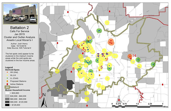
In 9-1, I again used fire station service calls data to look for hot and cold spots with the Cluster and Outlier Analysis tools. This was compared with the median household income data for the same area to determine if there was a relationship between income and service calls. In 9-2, I used the Hot Spot Analysis tool to find hot and cold spots in regards to income clustering. I conducted this analysis to find what areas were best to target for job creation compared to which were best for charity donations.

Figure 1. Diagram of methods.

Results

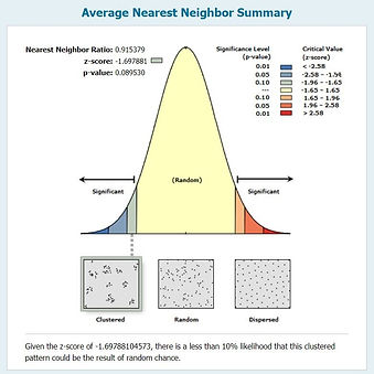
Figure 2. Average nearest neighbor summary for calls of service in February 2015.

Figure 3. Additional statistics from the average nearest neighbor summary illustrated in Fig. 2.

Figure 4. Map of nearest neighbor index for EMS calls for service.

Figure 5. Map of EMS calls for service call priority ranking.

Figure 6. Map of EMS calls for service spatial cluster analysis.

Figure 7. Map of library patron spatial autocorrelation analysis.

Figure 8. EMS calls for service cluster and outlier analysis.

Figure 9. EMS calls for service cluster and outlier analysis.

Figure 10. Map of income clustering hot spot analysis.

Application & Reflection

Problem Description: Spatial pattern analysis can have important applications in agriculture. For instance, some of the tools used here could be used to find hot spots for pests, diseases, or nutrient disorders. Farmers often apply treatments (i.e. fertilizers or pesticides) over an entire field to mitigate the issue. Unfortunately, this type of blanket treatment wastes a lot of time and resources, and can lead to issues of pesticide resistance in pests and pathogens. It would be of interest to track patterns of disease or pest occurrence within a field to locate hot spots and make more precise treatments.

Data Needed: To conduct this analysis, one would need to obtain data with points of known issues within an agronomic field.

Analysis Procedures: To analyze this, one would simply use the Average Nearest Neighbor tool to determine the distribution pattern. Based on the distribution (i.e. random, clustered or dispersed), one could do further analyses using some of the other tools. This application in spatial patterns could allow farmers to track areas of poor nutrition, or high disease or pest pressure to better manage crop management practices and optimize treatments.